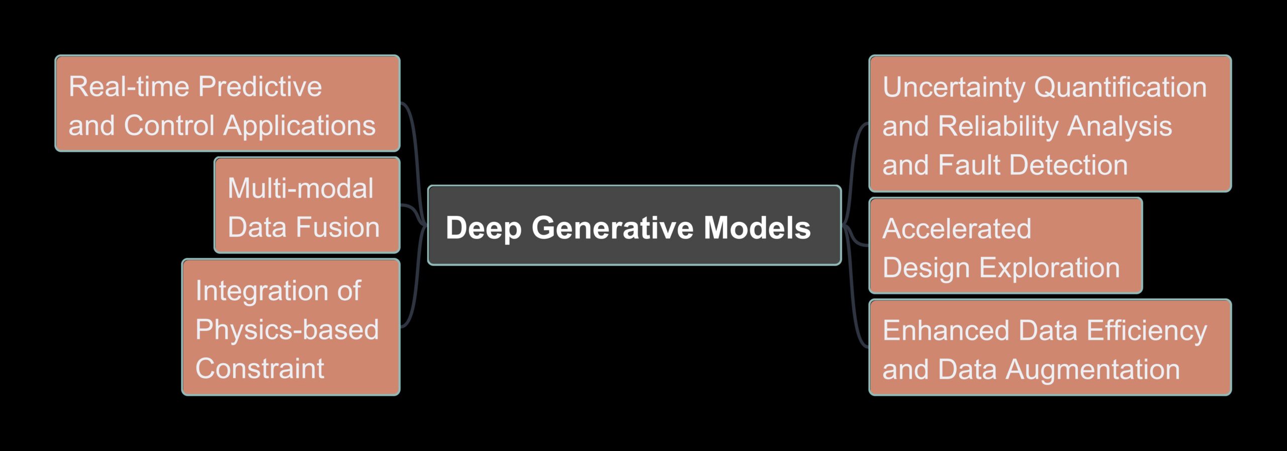
Artificial intelligence (AI) involves more than just decision-making; it encompasses understanding and generating data. Traditional discriminative models, tasked with classifying data into distinct categories, face challenges when noise is present, which can result in incorrect predictions. This points to a key limitation:

“AI systems need to not only classify data but also comprehend and generate it meaningfully.”

Deep Generative Models offer a solution by learning the underlying data distribution. These models allow AI systems to express uncertainty, making them more reliable in real-world applications. A crucial point raised is that current AI models, if unable to quantify uncertainty, may not be trustworthy, particularly in sensitive areas like medical diagnosis or autonomous driving.

Deep generative models have applications across various fields, including:

• Text, Image, and Audio Processing: For tasks like natural language generation, image synthesis, and speech enhancement.
• Active Learning: Selecting the most informative samples for labeling in machine learning.
• Reinforcement Learning: Simulating realistic environments for agents to learn optimal behaviors.
• Medical Imaging: Enhancing diagnosis by generating plausible medical images and improving interpretability.

Generative modeling is essential for AI systems, enabling them to model complex distributions and generate realistic outputs​. In fact, Deep generative modeling is a fascinating hybrid that combines probability theory, statistics, probabilistic machine learning, and deep learning in a single framework.

How to Formulate Deep Generative Modeling?

It is categorized into five major types:

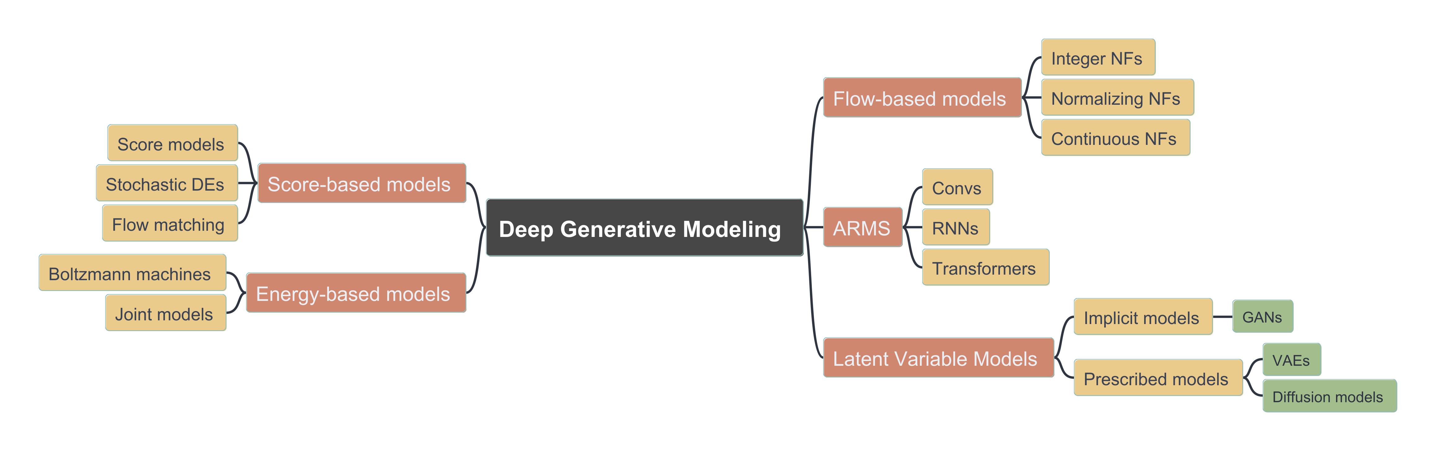
Latent Variable Models

Latent Variable Models describe the probability distribution of observed data using a mixture of unobserved (latent) variables. Mathematically, a latent variable model is defined as:²

$$ p_{\theta}(x)=\int{p_{\theta}(x|z)p(z)dz} $$

where:

\( p_\theta (x|z) \) is the likelihood function (the observation model),

\( p(z) \) is the prior distribution over the latent variables,

\( z \) is the latent variable that helps in capturing structured dependencies in data.

The challenge in training LVMs lies in computing the marginal likelihood \( p_\theta (x) \), which is generally intractable due to the integration over the latent space.

There are two primary approaches to leverage LVMs:

1. Neural Importance Sampling (NIS):

• Used to estimate partition functions in thermodynamics.
• Reduces variance in high-dimensional probability distributions.
• Applies importance sampling within latent variable inference to enhance accuracy.

2. Neural Markov-Chain Monte Carlo (NMCMC):

• A hybrid approach that combines MCMC with deep generative models.
• Utilizes LVMs to propose new samples and accelerate convergence in thermodynamic systems​.

1. Variational Autoencoders (VAEs):

To approximate the intractable posterior \( p(z|x) \), we can introduce a variational distribution \( q_{\phi}(z|x) \) and derive the Evidence Lower Bound (ELBO):

\[ \log p_{\theta}(x) \geq \mathbb{E}_{q_{\phi}(x|z)} \left[ \log p_{\theta}(x|z) \right] – D_{KL} \left( q_{\phi}(x|z) \parallel p(z) \right) \]

which is optimized during training.

where:

    First term: Reconstruction loss (ensures the generated sample \( x \) from \( p_\theta(x|z) \) is accurate).

    Second term: KL divergence (ensures a structured latent space).

the term:

\( D_{KL}(q_\phi(x|z) \parallel p(z)) \)

represents the Kullback-Leibler (KL) divergence between the variational posterior \( q_\phi(z|x) \) and the prior distribution \( p(z) \).

• It measures how different the approximate posterior \( q_\phi(z|x) \) (which is learned) is from the chosen prior \( p(z) \).
• The KL divergence acts as a regularization term that forces the latent variable distribution to stay close to the prior.

Why is it Important?

• Encourages structure in the latent space: It prevents overfitting by forcing the encoder distribution \( q_\phi(z|x) \)  to stay close to the prior \( p(z) \).
• Ensures smooth interpolation: The prior \( p(z) \) is usually chosen as \( \mathcal{N}(0, I) \) (a simple Gaussian), so minimizing the KL divergence ensures that the latent space is smooth and continuous.
• Regularizes the model: Without this term, the model could arbitrarily spread \( q_{\phi}(z) \)  over a complex space, making sampling unreliable.

2. Diffusion Models

Diffusion models are probabilistic generative models that learn to transform a simple noise distribution into a complex data distribution via a forward and reverse diffusion process.

1. Forward Diffusion Process

The forward diffusion process gradually adds noise to data over time following an Stochastic Differential Equation (SDE):

$$dx(t) = f(x, t)dt + g(t)dw(t)$$

• \( w(t) \) is a Wiener process (Brownian motion),
• \( f(x, t) \) is the drift coefficient, which controls deterministic transformations,
• \( g(t) \) is the diffusion coefficient, which scales the noise process.

As time progresses to a large value \( T \), the distribution \( p_T(x) \) converges to a known prior distribution, typically a Gaussian distribution \( \mathcal{N}(0, I) \).

2. Reverse Diffusion Process

To generate data, we reverse the forward diffusion process using a denoising SDE:

$$dx(t) = \left[ f(x, t) – g^2(t) \nabla_x \log p_t(x) \right] dt + g(t) d\bar{w}(t)$$

• \( \nabla_x \log p_t(x) \) is the score function, which helps guide the denoising process,
• \( \bar{w}(t) \) is a reverse-time Wiener process.

By solving this SDE numerically, we can generate realistic samples from the learned distribution.

3. Discretized Diffusion Process

The forward process can be discretized using a simple noise schedule:

$$x_t = \sqrt{\alpha_t} x_0 + \sqrt{1 – \alpha_t} \epsilon_t$$

where:

• \( \alpha_t \) is a sequence defined as \( \alpha_t= \prod_{\tau=1}^{t} (1 – \beta_\tau) \)
• \( \beta_\tau \) controls the noise schedule,
• \( \epsilon_t \) is standard Gaussian noise, \( \epsilon_t \sim \mathcal{N}(0, I)\).

The corresponding reverse process is:

$$x_{t-1} = \frac{x_t – (1 – \alpha_t) \nabla_x \log p(x_t)}{\sqrt{\alpha_t}} + \sqrt{1 – \alpha_t} \epsilon_t$$

which iteratively refines noisy samples to generate realistic data.

4. Probability Flow ODE

Instead of using an SDE, diffusion models can also be formulated using a Probability Flow Ordinary Differential Equation (ODE):

$$\frac{dx}{dt} = f(x, t) – \frac{1}{2} g^2(t) \nabla_x \log p_t(x)$$

which removes stochasticity and allows for deterministic sampling using numerical ODE solvers.

5. Training Objective

Diffusion models are trained using a denoising score-matching loss, where a neural network \( s_\theta(x, t) \) approximates \( \nabla_x \log p_t(x) \), the score function:

$$L(\theta) = \mathbb{E}_{x_0, t, \epsilon} \left[ \lambda(t) \| s_\theta(x_t, t) – \nabla_x \log p_t(x_t) \|^2 \right]$$

where \( \lambda(t) \) is a weighting function that stabilizes training.

Summary

• Diffusion models progressively refine noise into structured data.
• They use a forward diffusion process to gradually add noise and a reverse process to denoise.
• They can be formulated using stochastic differential equations (SDEs) or probability flow ODEs.
• Training involves learning a score function that approximates the noise removal process.

Flow-based Models

Flow-based generative models transform a simple probability distribution into a complex one using a sequence of invertible transformations. These models allow for exact likelihood estimation and efficient sampling.

1. Change of Variables Theorem

Flow-based models use the change of variables formula to compute the probability density function:

$$ p(x) = p(z) \left| \det J_f(z) \right|^{-1}$$

where:

• \( z=f^{-1} (x)\) is the latent variable transformed from \( x\).
• \( J_f(z)\) is the Jacobian matrix of the transformation \( f\).
• \( p(z) \) is the base distribution, typically \( \mathcal{N}(0, I) \).

2. Training Objective

The log-likelihood is derived as:

$$log p(x) = \log p(z) – \log \left| \det J_f(z) \right|$$

Maximizing this objective ensures that the model learns a transformation
\( f\) that maps simple distributions to complex data distributions.

3. Types of Normalizing Flows

Affine Coupling Layers

Affine coupling layers simplify the Jacobian computation while ensuring invertibility:

$$y_1 = x_1$$

$$y_2 = x_2 \odot \exp(s(x_1)) + t(x_1)$$

where \( s(x_1)\) and \( t(x_1)\) are scale and translation functions learned by a neural network.

Invertible ResNet Flows

ResNet flows use a residual connection to enforce invertibility:

$$y = x + g(x)$$

where \( g(x)\) is a constrained neural network ensuring \( \left|| \ J_g \right|| <1\), which guarantees invertibility​.

4. Continuous Normalizing Flows (CNFs)

Instead of discrete transformations, CNFs define transformations via Ordinary Differential Equations (ODEs):

$$\frac{dz}{dt} = f_{\theta}(z, t)$$

The density evolution follows the Instantaneous Change of Variables:

\[ \frac{d \log p(z | t)}{dt} = – \text{tr} \left( \frac{\partial f_{\theta}(z, t)}{\partial z} \right) \]

This avoids computing Jacobian determinants directly, making CNFs scalable for high-dimensional data.

Score-based Models

Score-based generative models learn to generate data by estimating the score function (gradient of the log probability density) and using it to guide sampling via Langevin dynamics or stochastic differential equations.³

1. Score Function and Its Estimation

The score function of a probability distribution \( p(x) \) is defined as:

$$s(x) = \nabla_x \log p(x)$$

where \( s(x) \) represents the gradient of the log-density with respect to \( x \). Instead of learning the density function directly, score-based models learn an approximation \( s_{\theta}(x) \) using score matching.

2. Denoising Score Matching Objective

To train a score-based model, we use denoising score matching, where a noise-perturbed version \( \tilde{x}\) of the data \( x \) is introduced:

$$L(\theta) = \mathbb{E}_{x, \epsilon} \left[ \lambda(\sigma) \left\| s_{\theta}(\tilde{x}) + \frac{\epsilon}{\sigma} \right\|^2 \right]$$

where:

• \( \tilde{x}= x+ \sigma\epsilon \) with \( \epsilon \sim \mathcal{N}(0, I) \) (Gaussian noise),
• \( \lambda(\sigma) \) is a weighting function that stabilizes training.

3. Langevin Dynamics for Sampling

Once the score function is learned, data samples can be generated using stochastic gradient Langevin dynamics (SGLD):

$$x_{t+1} = x_t + \eta s_{\theta}(x_t) + \sqrt{2 \eta} \xi_t$$

where:

• \( \eta \) is the step size,
• \( \xi_t \sim \mathcal{N}(0, I)\) is Gaussian noise.

This process iteratively refines a random initialization into a sample from \( p(x) \).

4. Stochastic Differential Equation (SDE) Formulation

The Stochastic Differential Equation (SDE) Formulation in Score-Based Models and the Forward Diffusion Process formulation in Diffusion Models share the same general form because diffusion models are a special case of score-based models.

• Diffusion models use the forward SDE to define the process of adding noise.
• Score-based models use the same equation to define the reverse process, leveraging the score function to undo the noise addition.

Thus, score-based models generalize diffusion models, as diffusion models implicitly estimate the score function while score-based models explicitly learn it.

Key Difference:

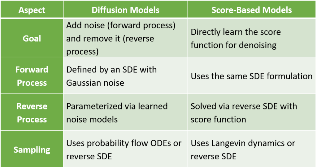
Generally, both models rely on stochastic differential equations (SDEs) to describe the transformation of data, but diffusion models use it explicitly for noise injection, while score-based models leverage it to learn the probability distribution gradient (score function) for sampling.

Here is a comparison of the five types of generative models across four aspects:

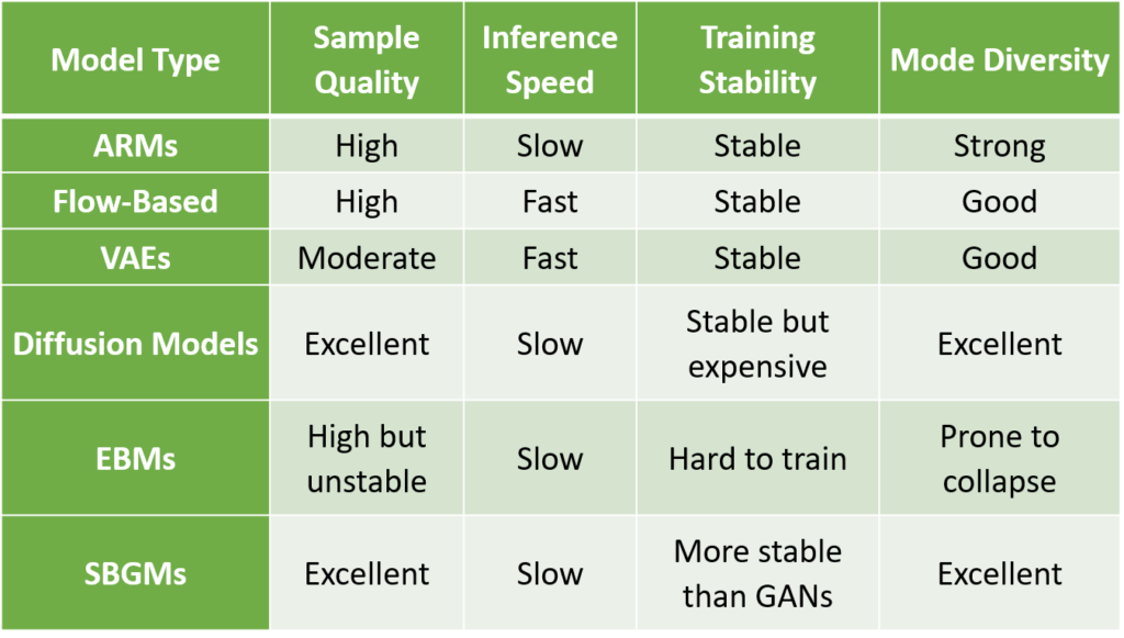
Each model class has trade-offs, with Flow-Based Models excelling in speed, Diffusion and Score-Based Models in quality and mode diversity, and Autoregressive Models in likelihood-based generative capabilities. Your choice depends on the application.

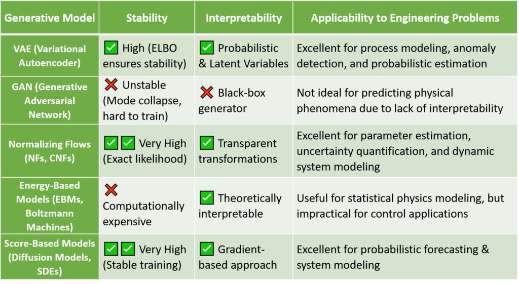
For engineering applications, such as chemical process control, high-dimensional systems, and probabilistic modeling, the choice between VAEs, GANs, Flow-Based Models, Energy-Based Models, and Score-Based Models depends on the stability, interpretability, and generalizability of each approach. Here’s a comparative analysis:

1. Stability & Reliability for Engineering Applications:

2. Best Choice for Different Engineering Scenarios:

2.1. Chemical Process Control Engineering

Best Choice: VAEs & Normalizing Flows (CNFs)

Why?

Chemical processes are stochastic and high-dimensional. So, VAEs capture latent variables useful for state estimation, while CNFs provide an exact probability density function.
Examples:

• Predicting fault detection & sensor calibration.
• Building a surrogate model for Model Predictive Control (MPC).
• Estimating reaction kinetics in multiphase reactors.

GANs & EBMs are less suitable:

• GANs do not guarantee probability density estimation.
• EBMs require expensive MCMC sampling, making them impractical.

2.2. High-Dimensional Systems (e.g., Fluid Dynamics, Power Systems)

Best Choice: Score-Based Generative Models (Diffusion Models) & Normalizing Flows

Why?

Score-based models (SDE-based) model high-dimensional distributions more accurately than VAEs or GANs.
Examples:

• Model reduction for turbulent flow simulations.
• Uncertainty quantification in power grids.
• Real-time optimization in dynamic systems.

VAEs can be useful for reducing dimensionality before applying physics-informed models.

2.3. Probabilistic Systems (e.g., Bayesian Calibration, Stochastic Optimization)

Best Choice: VAEs & Flow-Based Models

Why?

Engineering problems often require probability density estimation, which VAEs and Normalizing Flows handle well.
Examples:

• Bayesian inverse modeling in material design.
• Risk-aware control in industrial automation.

Score-Based Models can be useful for generating high-quality posterior samples in Bayesian inference.

Key Points:

• VAEs are the most stable and interpretable for process control, anomaly detection, and uncertainty quantification.
• Normalizing Flows (CNFs) are superior for high-dimensional engineering models and probabilistic inference.
• Score-Based Generative Models are excellent for complex, high-dimensional simulations (e.g., fluid flow, energy grids).
• GANs and EBMs are less suitable for engineering applications due to unstable training and computational cost. So, Avoid GANs unless high-quality sample generation is needed.

References:

1. Tomczak, J.M., 2024. Deep Generative Modeling. Springer International Publishing, Cham. https://doi.org/10.1007/978-3-031-64087-2 ↩︎
2. Nicoli, K.A., n.d. Deep Generative Models for Thermodynamics of Spin Systems and Field Theories. ↩︎
3. Bergamin, F., n.d. Advances in Deep Generative Models, Approximate Inference, and their Applications. ↩︎